PPO is the most widely used policy gradient algorithm in deep reinforcement learning. It trained OpenAI Five to beat the Dota 2 world champions in 2019, the robot hand that solved a Rubik’s cube that same year, and the RLHF step behind InstructGPT and ChatGPT in 2022.
Most explanations show the PPO objective in full and then work backwards. Here we build it up one term at a time, so that nothing appears without a reason.
PPO is really just a few additions to REINFORCE, an algorithm from 1992. REINFORCE is about as simple as a learning algorithm gets: a dozen lines of code.
The whole idea is one sentence: run your policy, see which episodes went well, and make those actions more likely.
1 · On-policy RL, in its simplest form
An agent acts, collects rewards, and the episode ends. We want whatever behavior collects the most reward.
All of that behavior lives in the policy , one neural network with weights . Handed a state it returns a probability distribution over actions, .
One pass through the environment leaves a trail of states, actions and rewards. Call it a trajectory:
How good was the episode? Add up the rewards, optionally shrinking later ones by a factor per step so that reward now counts for more than reward later. That sum is the return :
✎ Exercise 1 · the return of a trajectory
The return of one whole episode: a single number, not one per step.
# rewards : torch.Tensor (T,)    reward at each step of one episode
# gamma   : float                discount factor
# ->        torch.Tensor scalar  the return of the whole episode
def trajectory_return(rewards, gamma):
  ...
torch.arange(len(rewards)) gives you [0, 1, 2, ...], and gamma ** x is a tensor you can multiply through elementwise before calling .sum().A plain Python loop over
enumerate(rewards) works just as well.The objective is the expected value of the return, for a trajectory sampled from the policy. Call it :
We want to find the policy that maximizes .
is a neural network, so maximizing means gradient ascent, which requires . Luckily, this identity lets us compute it:
A gradient of an expectation becomes an expectation of a gradient, and those you can estimate by sampling. This is the score function estimator.
Apply it to , with :*
A working algorithm, and a naive one.
Reading it carefully says why: every action in the episode is multiplied by the same number . An action taken at step is credited with rewards collected at step .
2 · REINFORCE
An action cannot influence rewards that arrived before it. That is the principle of causality. Those earlier terms are not signal; they are noise, added to every update that action will ever receive. So we credit each action with only what came after it. That is the REINFORCE reward:
Swapping it in costs nothing: the discarded terms had expectation zero, so the estimator is still exactly unbiased, and strictly quieter. This is REINFORCE in the form people usually mean:
Notice what actually is. It is the observed return, a sum of rewards that really happened, not an estimate of anything. REINFORCE has no value function, no model of the environment, nothing to learn but the policy itself.
✎ Exercise 2 · reward-to-go
The sum above has an equivalent recursive form, and it is the one you want here:
Walk backwards and each return is one multiply and one add. The loop is written for you. Fill in the line that carries the return back a step.
# rewards : torch.Tensor (T,)    reward at each step of one episode
# gamma   : float                discount factor
# ->        torch.Tensor (T,)    G[t] = return from step t onwards
def reward_to_go(rewards, gamma):
  G = torch.zeros_like(rewards)
  acc = 0.0
  for t in reversed(range(len(rewards))):
      acc = ...
      G[t] = acc
  return G
acc is read versus when it is written. On the right-hand side it still holds the value from the previous iteration, and since you are walking backwards, that previous iteration was step t+1.Whichever action you sample goes up
One state, three actions. We sample an action and collect the reward it pays. The episode is one step long, so .
Set what each action returns and choose which one came out of the sample. The bars show where the probabilities end up.
Every action returns something positive, so only the one that gets sampled is reinforced, even the worst of the three.
3 · REINFORCE minus a baseline
If every is positive then every action is pushed up, and only the differences between them carry any information.
The fix is to subtract a reference point. Call it the baseline, :
The surprising part is that you may choose it freely: any such leaves the gradient’s expectation exactly where it was.
The reason is worth seeing without the algebra too. Probabilities in a state sum to one, so pushing all of them up by the same amount pushes none of them up relative to each other.
The best baseline is the one that predicts the return you were about to get: , the value of being in state .
The same three actions. Let’s replace with .
The return is measured against that average now, so a sampled action can be pushed down, not just up.
4 · One equation to rule them all
Look back at what actually changed between the last three formulas. The factor never moved. Only the number multiplying it did.
So give that coefficient a name and write the family once:
Every algorithm from here (A2C, TRPO, PPO) is a choice of .*
| REINFORCE, naive | |
| + causality | |
| + baseline | |
| A2C | coming next |
| PPO | coming next |
5 · A2C
Three additions: bootstrapping, the critic (a second neural network, estimating ), and GAE.
Bootstrapping
Using means waiting for the episode to end. But you do not need the whole episode to judge an action. The value of a state is the reward you collect plus the value of wherever you land. That is the Bellman equation:
So stop after one step: take the reward you got and let the value of the next state stand in for the rest.
We do not have . In its place put a second network, , with its own parameters , trained to predict what a state is worth.
The gap between what predicted and what one step of reality says is the TD error, .
We are improving an estimate using another estimate. That is bootstrapping, and it is the one idea separating A2C from everything before it.
✎ Exercise 3 · the TD error
One line, no loop. The only catch is : for every step it is the next
entry of values, and the last step has no next entry, so last_value stands in for it.
# rewards    : torch.Tensor (T,)  reward collected at each step of the rollout
# values     : torch.Tensor (T,)  the critic's V(s_t) at each step
# last_value : torch.Tensor ()    the critic's V(s_T), where the rollout stopped
# gamma      : float
# ->           torch.Tensor (T,)  one TD error per step
def td_error(rewards, values, last_value, gamma):
  ...
values[1:] is V(s_t+1) for every step but the last. torch.cat joins it with last_value.reshape(1) to cover that one. Then subtract values.The critic
There are two networks now, doing different jobs. picks actions: it is the actor, and the only part that gets used once training is over. never chooses anything. It predicts, and its prediction is what the actor’s choices get measured against. It is the critic.
And the quantity being measured has a name. How much better an action turned out than what the policy would have done on average is the advantage:
It is zero-mean under the policy, , so better-than-average actions get positive weight and worse-than-average get negative. Section 3’s baseline was already estimating it with a whole episode; estimates it with one step.
Three words, three pieces. A2C is advantage actor-critic.
The gain is less variance: one transition’s worth of noise instead of an entire episode’s, and no waiting for the episode to end, since a single step is now enough to learn from.
The cost is correctness. is an advantage estimate only when , and is never quite right, so where every estimator so far was unbiased and merely noisy, this one is biased.
GAE
We now have two estimates of the same advantage, and they disagree about how far to look before trusting the critic.
- REINFORCE (Monte Carlo) waits for the entire episode: no bias, a great deal of noise.
- The TD error looks one step ahead: very little noise, some bias.
Nothing forces that choice. You could take two real rewards before falling back on , or three, or ten:
So rather than picking one, take a weighted average of all of them, with the weight decaying by a factor each step further out. That average collapses into a single sum over the TD errors we already have:
This is the generalized advantage estimator, and is the dial.
At nothing decays: Monte Carlo again.
At only the first term survives: the single TD error. The two algorithms we have built so far are the same one, at opposite ends of this dial.
So which setting? In practice almost everyone picks — close to the Monte Carlo end, but not quite at it. The plot below shows why.
✎ Exercise 4 · GAE
One line. delta is already there: the TD error at this step. What is left is acc,
which carries it backwards, and that is the whole of GAE: the same accumulation you
wrote in exercise 2, with a second decay on it.
# rewards    : torch.Tensor (T,)     reward at each step
# values     : torch.Tensor (T,)     V(s_t), the critic at each step
# last_value : torch.Tensor scalar   V(s_T), to bootstrap the final step
# gamma, lam : float
# ->           torch.Tensor (T,)     the GAE advantage at each step
def gae(rewards, values, last_value, gamma, lam):
  adv = torch.zeros_like(rewards)
  acc = 0.0
  for t in reversed(range(len(rewards))):
      v_next = last_value if t == len(rewards) - 1 else values[t + 1]
      delta = rewards[t] + gamma * v_next - values[t]
      acc = ...
      adv[t] = acc
  return adv
acc = rewards[t] + gamma * acc. The shape here is identical: this step's quantity, plus a decayed copy of what acc already held.Only two things change. The quantity is
delta rather than the raw reward, and the decay is gamma * lam rather than gamma.6 · PPO
A2C uses each transition once and throws it away. After a single gradient step , so the batch was produced by a policy we no longer have, and the on-policy expectation from section 1, which assumed the data came from the policy being updated, no longer applies.
Weight each sample by how much more likely the new policy is to have taken it:
and the objective is usable again:
Reweighting samples drawn from one distribution in order to estimate an expectation under another is called importance sampling; is the importance weight. Here it is what makes a second pass over the same batch legitimate.
A quick check that nothing was smuggled in: at the very start of the update , so and the gradient is exactly A2C’s.
✎ Exercise 5 · the importance ratio
You have logp_new and logp_old. Log probabilities are what a policy
actually returns. Produce , elementwise.
# logp_new : torch.Tensor (N,)  log pi_theta(a|s), the policy being updated
# logp_old : torch.Tensor (N,)  log pi_old(a|s), the one that collected the batch
# ->         torch.Tensor (N,)  one ratio per sample
def importance_ratio(logp_new, logp_old):
  ...
torch.exp. Two operations, no loop.There is a catch, though. Nothing bounds . With the objective grows without limit as , so gradient ascent will happily drive one sampled action’s probability to 1 on the strength of a single batch.
Say took an action with probability and now takes it with probability . Then , and that single sample pulls nine times as hard as it did when it was collected.
We need to constrain how far the policy may move in one update. The principled way is to bound the KL divergence between and — a measure of how far apart two distributions are. An improvement guarantee can be proved mathematically when using KL divergence.
TRPO, for trust region policy optimization, is the 2015 algorithm PPO grew out of, and it uses the KL directly: maximize the objective subject to .
That works, but it is expensive.
PPO approximates that constraint inside the objective itself, by clipping the ratio so that moving too far stops paying:
If that looks intimidating, there are only two cases — one per sign of :
| advantage | ratio | ||
|---|---|---|---|
| gradient flows | |||
| gradient zero | |||
| gradient flows | |||
| gradient zero |
✎ Exercise 6 · the clipped surrogate
From ratio, adv and clip_coef, return the scalar loss. Two traps: the
leading sign, and which of min/max you need.
# ratio     : torch.Tensor (N,)      pi_theta / pi_old, one per sample
# adv       : torch.Tensor (N,)      advantage estimate, one per sample
# clip_coef : float                  epsilon, e.g. 0.2
# ->          torch.Tensor scalar    the LOSS (a negated objective)
def clipped_surrogate(ratio, adv, clip_coef):
  ...
torch.min(a, b) takes the elementwise minimum of two tensors, not .min(), which reduces a single one. .clamp(lo, hi) is the clip itself. Then .mean() over the batch.On the sign: PPO maximizes the surrogate, and optimizers minimize.
Clipping allows PPO to reuse data
What PPO adds is data reuse: several gradient steps on each batch instead of one. The ratio is what makes that legitimate, since a batch collected under still counts for the policy we have now. The clip is what keeps those extra steps safe. Neither data reuse nor clipping does anything alone. Let’s run both on the same environment.
Cliff Walking is a small gridworld: per step, for stepping off the cliff, and an optimal route worth .
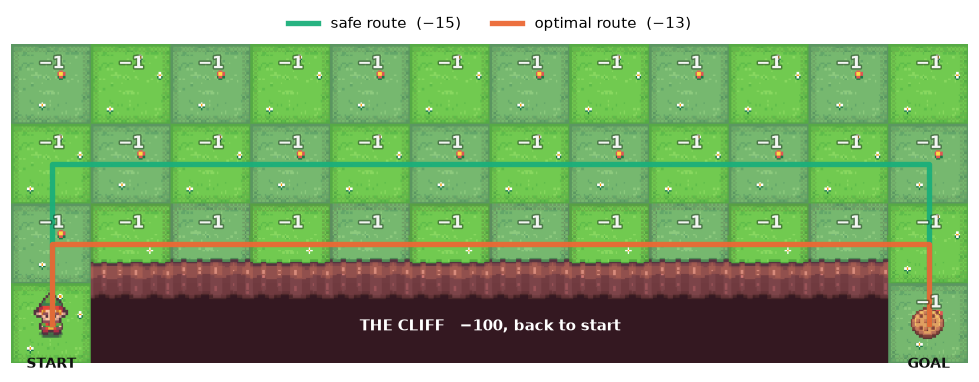
Run at for 400k environment steps, it defeats A2C completely. Every row below sees that same amount of experience; only the update changes:
| gradient steps per rollout | clip | return | |
|---|---|---|---|
| 1 | off | −1338 | |
| 1 | 0.2 | −1338 | identical: with the clip is inert |
| 16 (4 epochs × 4 minibatches) | off | −676 | overshoots |
| 16 | 0.2 | −14 | solved |
Sixteen times the learning per unit of experience is what lets the policy find the goal, and the clip is what stops sixteen unconstrained steps on one batch from blowing up.
Why is what breaks A2C here is worth its own look. Bootstrapping needs the Bellman backup to be a contraction, and is the contraction modulus. At there is no fixed point to fall into at all:
The whole loss
Everything so far has been the policy term. A real implementation adds two more:
The critic term trains : plain regression onto the returns the rollout actually produced, .
The entropy term pays the policy to stay spread out. is largest when it still gives every action a chance and zero once it always picks the same one, so rewarding it delays the moment exploration stops.
✎ Exercise 7 · put it together
The three terms are computed for you. Combine them into the single scalar that gets differentiated.
# pg_loss  : torch.Tensor scalar   clipped surrogate, already negated
# v_loss   : torch.Tensor scalar   mean squared error of the critic
# entropy  : torch.Tensor (N,)     H(pi) at each state in the batch
# vf_coef  : float                 weight on the critic
# ent_coef : float                 weight on exploration
# ->         torch.Tensor scalar   the one number you call .backward() on
def ppo_loss(pg_loss, v_loss, entropy, vf_coef, ent_coef):
  policy_term  = pg_loss
  value_term   = vf_coef * v_loss
  entropy_term = ent_coef * entropy.mean()
  return ...
pg_loss and v_loss are already errors, so they go in as they are.Entropy is the odd one out: high entropy is good, so to reward it inside something being minimized you have to subtract it.
And that is PPO — the whole objective, nothing held back. You derived it: the return, the reward-to-go, the baseline, the advantage, bootstrapping, GAE, the importance ratio, the clip. Every term above is something you built a reason for.
Every step, in one table
| bias | variance | needs full episodes | ||
|---|---|---|---|---|
| REINFORCE, naive | none | terrible | yes | |
| + causality | none | high | yes | |
| + baseline | none | moderate | yes | |
| A2C | yes | low | no | |
| PPO | yes | low | no |
The first two rows are free: variance down, bias unchanged. Only the move to A2C costs something, and it is the same thing every time: a target that refers to its own estimate. That is what buys the sample efficiency, and it is what breaks when .
NB — The last row is more than just a coefficient. PPO keeps A2C’s and changes what you may do with it: reuse the batch, so long as the policy does not wander too far while you do.Where to go next
The same path, further on. TRPO is the step PPO approximates: a hard KL constraint with a monotonic-improvement guarantee inherited from Conservative Policy Iteration. GAE is the dial in its own paper. GRPO drops the critic and returns to a Monte Carlo estimator with an empirical group-mean baseline — section 3, rediscovered for language models.
Exploration is its own field. RND and ICM supply the directed exploration sampling cannot; Go-Explore attacks it by remembering promising states; the noisy-TV problem is where curiosity itself breaks.
Off-policy avoids throwing data away at all. SAC for continuous control, and the deadly triad for why that is harder than it sounds.
Canonical sources. Sutton & Barto, Reinforcement Learning: An Introduction. Ch. 13 for policy gradients. The 37 Implementation Details of PPO for everything the equations leave out, and CleanRL for single-file implementations worth reading start to finish.